Exploring vaccine effectiveness through bayesian regression -- Part 4

Last time

Last time we paid homage to Doing Bayesian Data Analysis by Dr. John K. Kruschke (hereafter, simply DBDA) while exploring overall effectiveness of the Pfizer vaccine.

This time we’ll revisit brms and STAN which we touched upon in part 2. At the time I wrote:

Quite frankly it is more than we need for our simple little analysis. A bit like using a sledge hammer as a fly-swatter. Besides the simple joy of learning about it however, there is one practical reason to use it. As our data grows and we inevitably want to conduct more sophisticated analysis factoring things in like gender, age and race. It is likely to become the tool of choice.

Since the Pfizer data includes some early glimpses at information about factors such as age and race we can put brms to much better use this time. First step let’s load some packages.

library(dplyr)
library(brms)
library(ggplot2)
library(kableExtra)
theme_set(theme_bw())

What we know. Approximately 25,650 in the study (well at least eligible so far). Two age categories (Less than 65, or older than that). We can safely assume they are not evenly distributed across age groups, but are more or less equal in the number who received the true vaccine versus the placebo. 95 subjects contracted COVID, the rest did not. Of those 95 only 5 received the true vaccine yielding an effectiveness of ~ 94%. We don’t know from the press releases what the proportion by age was. But we can have some fun playing with the numbers and preparing for when we see fuller data.

One area of interest will no doubt be whether the vaccine protects older people as well as younger. So we’ll have two factors vaccine/placebo and <65 versus >= 65. For each of those we’ll have data on the number of people who got COVID and those who didn’t.

For our purposes we’re making some numbers up! They’ll be realistic and possible given the limitations I laid out above (for example only 5 people regardless of age got the true vaccine and got COVID). I’m going to deliberately assign a disproportionate number of the positive true vaccine cases to the older category a 4/1 split. Here’s a table, of our little dataframe agg_moderna_data.

Edit Nov 18th – I’m also aware that Pfizer has released even more data today that the vaccine is nearly equally effective for older people. But since I don’t have access to the exact numbers (if anyone has them send them along) we’ll make some up.

Table 1: Notional Moderna Data

Factors of interest		COVID Infection		Total subjects
condition	age	didnot	got_covid	subjects
placebo	Less than 65	8271	79	8350
placebo	Older	4494	11	4505
vaccinated	Less than 65	8293	1	8294
vaccinated	Older	4497	4	4501

Those familiar with frequentists methods in r will recognize this as an opportunity for glm. For reasons I’ll explain later I would prefer to use the aggregated data, although glm is perfectly happy to process as a long dataframe. So we’ll create a matrix of outcomes called outcomes with successes got_covid and failures didnot.

For binomial and quasibinomial families the response can be specified … as a two-column matrix with the columns giving the numbers of successes and failures

Voila the results using the native print function as well as broom::tidy. With classic frequentist methodology we can now “reject” the null that the \(\beta\) coefficients are 0. Both the main effects condition and age are significant as well as the interaction age:condition. Telling us that we must look at the combination of age and vaccine status to understand our results.

outcomes <- cbind(as.matrix(agg_moderna_data$got_covid, ncol = 1), 
             as.matrix(agg_moderna_data$didnot, ncol = 1))

moderna_frequentist <-
   glm(formula = outcomes ~ age + condition + age:condition,
       data = agg_moderna_data,
       family = binomial(link = "logit"))

moderna_frequentist

## 
## Call:  glm(formula = outcomes ~ age + condition + age:condition, family = binomial(link = "logit"), 
##     data = agg_moderna_data)
## 
## Coefficients:
##                  (Intercept)                      ageOlder  
##                       -4.651                        -1.362  
##          conditionvaccinated  ageOlder:conditionvaccinated  
##                       -4.372                         3.360  
## 
## Degrees of Freedom: 3 Total (i.e. Null);  0 Residual
## Null Deviance:       121.2 
## Residual Deviance: 5.18e-13  AIC: 23.71

broom::tidy(moderna_frequentist)

## # A tibble: 4 x 5
##   term                         estimate std.error statistic   p.value
##   <chr>                           <dbl>     <dbl>     <dbl>     <dbl>
## 1 (Intercept)                     -4.65     0.113    -41.1  0        
## 2 ageOlder                        -1.36     0.322     -4.22 0.0000240
## 3 conditionvaccinated             -4.37     1.01      -4.34 0.0000140
## 4 ageOlder:conditionvaccinated     3.36     1.16       2.89 0.00389

Notice that the \(\beta\) values are not especially informative because they are in link = “logit” format. We can infer direction. Older people, even though vaccinated still get COVID at higher rates. As we investigate bayesian methods we’ll convert back to our original scale. But let’s pause for a minute and acknowledge the limitations of the frequentist (NHST) method.

Things we can’t do (great reading here):

1. Claim that we are highly confident about our results because the p value is is very small? NO while you could construct confidence intervals around our \(\beta\) values you can’t make statements about probability, you either reject the null at some \(\alpha\) level or you don’t.

2. If the results were non-significant can you “accept” the null or say there is evidence for it. NO again that’s not permitted in the NHST framework.

3. Append this data to results from the study two months from now when the case count is higher? Another NO you can not legitimately keep adding data in a frequentist’s world.

A bayesian approach

brms is great package that very much mirror’s the way glm works. It abstracts away many of the stumbling blocks that newcomers find difficult about STAN and bayesian modeling in general.

Let me back up a minute. The simplest way to run the bayesian analog if our data were in long format i.e. we had a dataframe with 25,650 rows one per subject, would be the following command.

brm(data = moderna_long_data,
            family = bernoulli(link = logit),
            y ~ age + condition + age:condition,
            iter = 12500, warmup = 500, chains = 4, cores = 4,
            control = list(adapt_delta = .99, max_treedepth = 12),
            seed = 9,
            file = "moderna_long")

We’re treating COVID-19 outcomes as simple bernoulli events (a coin flip if you will). I’m providing the code so you can try it if you like. But I don’t recommend it. Expect a wait of 5 minutes or more!

Let’s go with a plan that works for the impatient (ME!). brm allows us to specify the outcomes aggregated. For each row of agg_moderna_data it’s got_covid | trials(subjects) or the number who became infected by the number of subjects in that condition. Again our \(\beta\)’s are in logit but we’ll correct that in a minute.

Notice file = "moderna_bayes_full" which saves our results to a file on disk named moderna_bayes.rds. That’s a blessing because we have the results saved and can get them back in a future session. But be careful if you rerun the command without deleting that file first it won’t rerun the analysis. We increased the default number of chains and iterations and after burn-in have 48,000 usable samples.

moderna_bayes_full <- 
   brm(data = agg_moderna_data,
       family = binomial(link = logit),
       got_covid | trials(subjects) ~ age + condition + age:condition,
       iter = 12500, 
       warmup = 500, 
       chains = 4, 
       cores = 4,
       seed = 9,
       file = "moderna_bayes_full")

summary(moderna_bayes_full)

##  Family: binomial 
##   Links: mu = logit 
## Formula: got_covid | trials(subjects) ~ age + condition + age:condition 
##    Data: agg_moderna_data (Number of observations: 4) 
## Samples: 4 chains, each with iter = 12500; warmup = 500; thin = 1;
##          total post-warmup samples = 48000
## 
## Population-Level Effects: 
##                              Estimate Est.Error l-95% CI u-95% CI Rhat Bulk_ESS
## Intercept                       -4.66      0.11    -4.88    -4.44 1.00    42732
## ageOlder                        -1.39      0.33    -2.08    -0.79 1.00    21396
## conditionvaccinated             -4.80      1.21    -7.73    -2.98 1.00    11248
## ageOlder:conditionvaccinated     3.72      1.35     1.45     6.80 1.00    12007
##                              Tail_ESS
## Intercept                       36581
## ageOlder                        21752
## conditionvaccinated             10470
## ageOlder:conditionvaccinated    11430
## 
## Samples were drawn using sampling(NUTS). For each parameter, Bulk_ESS
## and Tail_ESS are effective sample size measures, and Rhat is the potential
## scale reduction factor on split chains (at convergence, Rhat = 1).

bayestestR::describe_posterior(moderna_bayes_full, 
                               ci = 0.95, 
                               test = c("p_direction"),
                               centrality = "MAP")

## # Description of Posterior Distributions
## 
## Parameter                    |    MAP |           95% CI |      pd |  Rhat |       ESS
## --------------------------------------------------------------------------------------
## Intercept                    | -4.651 | [-4.884, -4.437] | 100.00% | 1.000 | 42708.798
## ageOlder                     | -1.357 | [-2.050, -0.769] | 100.00% | 1.000 | 21032.449
## conditionvaccinated          | -4.166 | [-7.274, -2.760] | 100.00% | 1.001 |  9684.929
## ageOlder.conditionvaccinated |  3.285 | [ 1.308,  6.549] |  99.96% | 1.001 | 10879.160

Notice how similar our results are to glm. We can also use bayestestR::describe_posterior directly on the brmsfit object.

One of the very nice things about brms is that it has plot methods for almost everything you might want to plot. A few examples below and even more commented out.

mcmc_plot(moderna_bayes_full)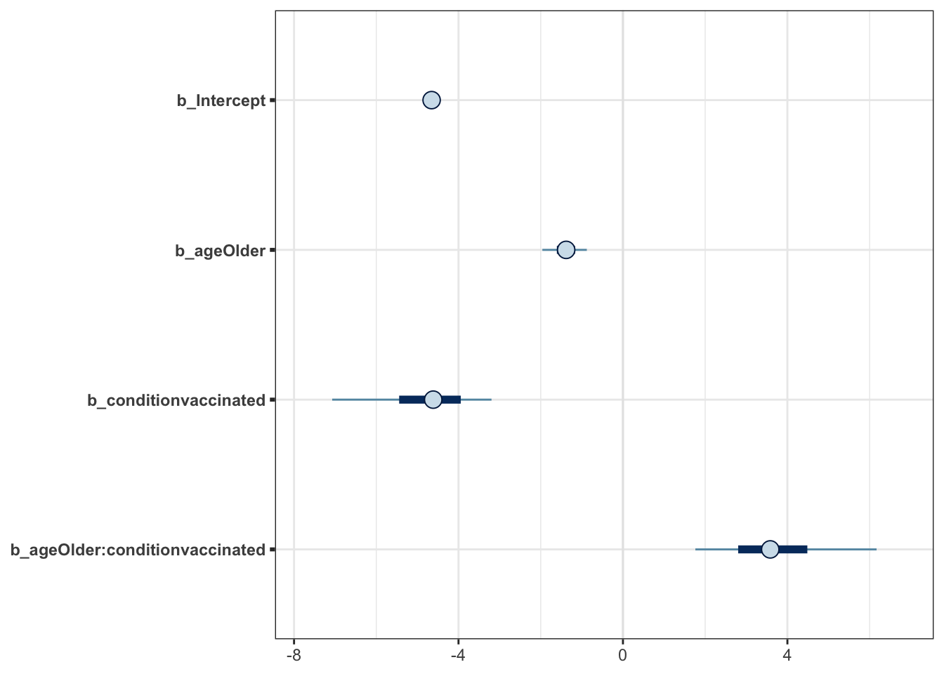

mcmc_plot(moderna_bayes_full, type = "areas")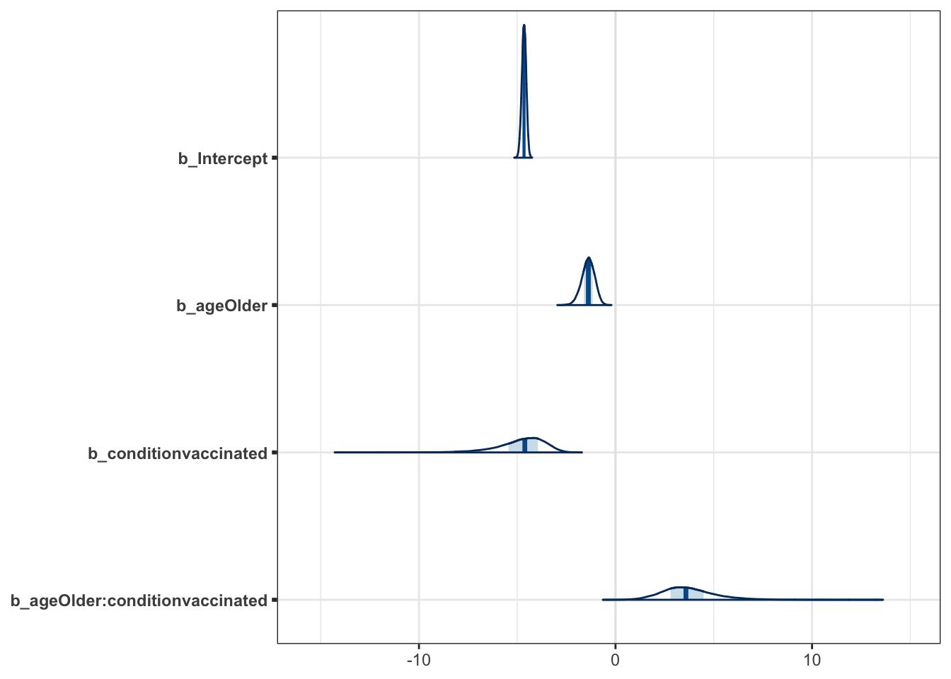

mcmc_plot(moderna_bayes_full, type = "trace")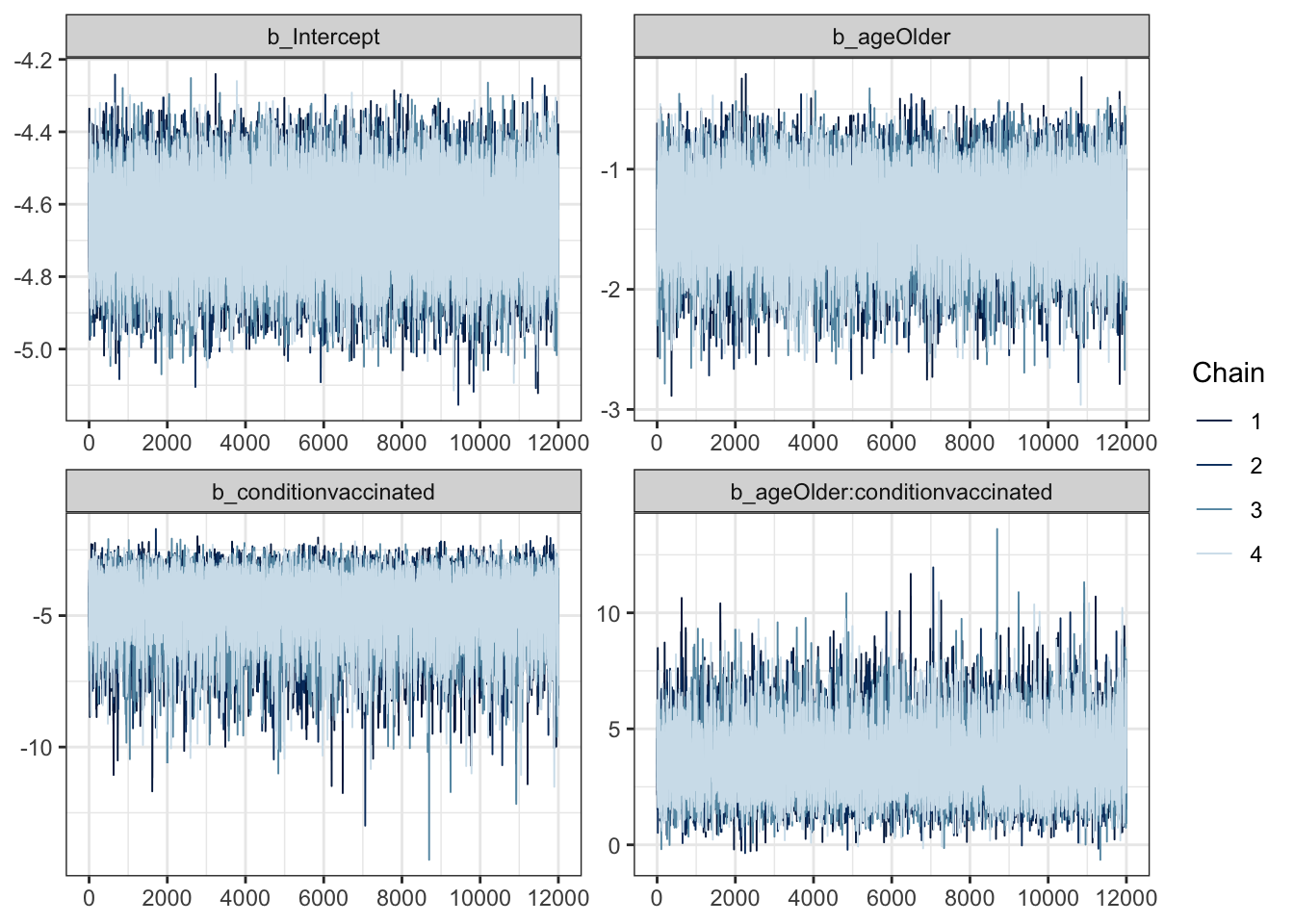

mcmc_plot(moderna_bayes_full, type = "hist")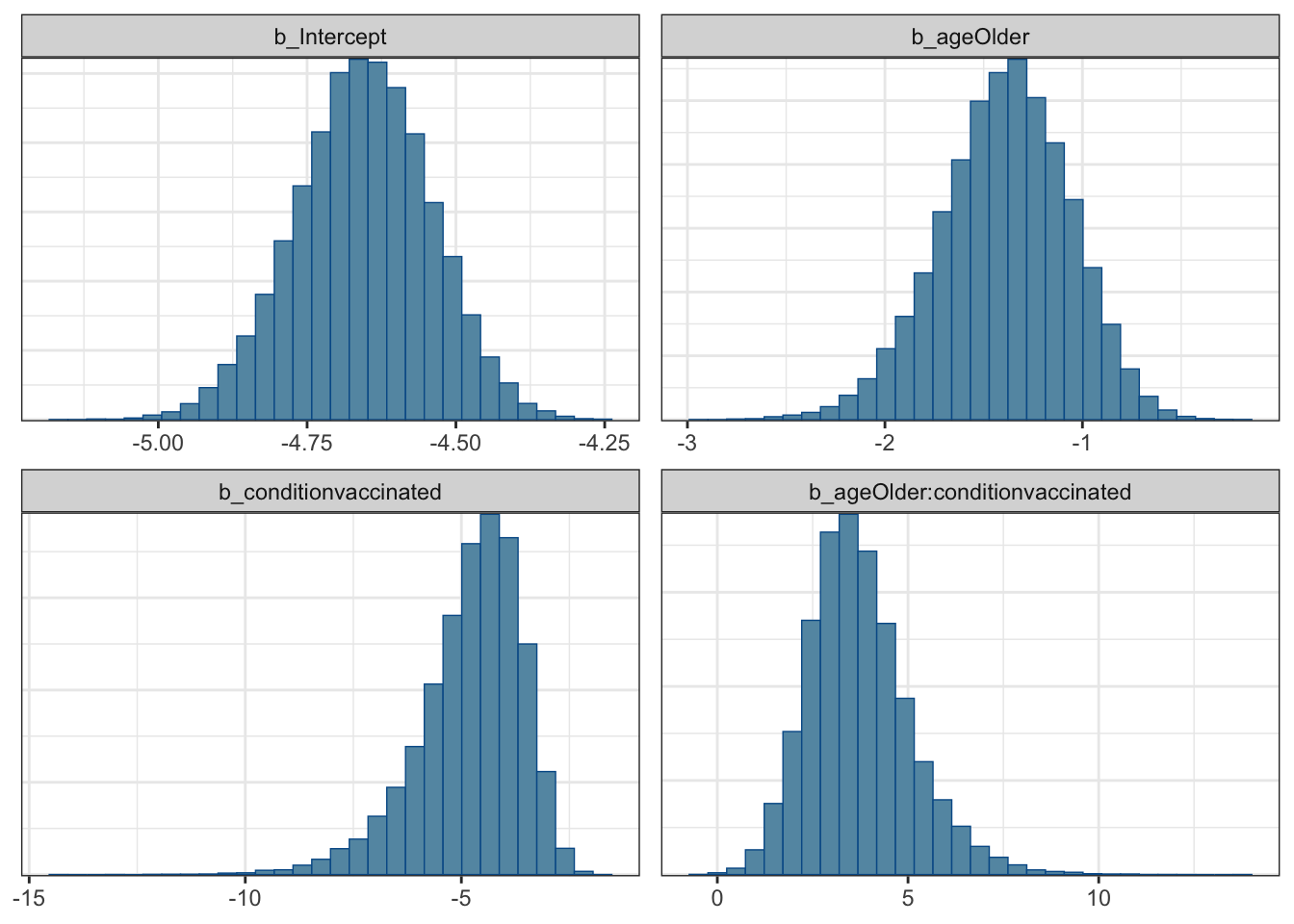

mcmc_plot(moderna_bayes_full, type = "dens_overlay")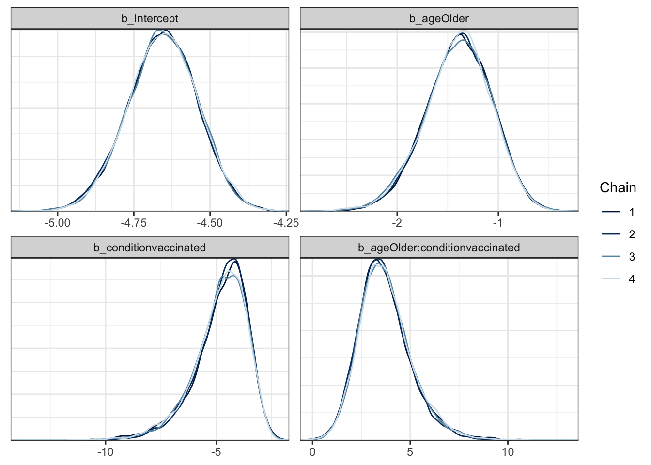

# mcmc_plot(moderna_bayes_full, type = "acf")
# mcmc_plot(moderna_bayes_full, type = "neff")
# mcmc_plot(moderna_bayes_full, type = "nuts_treedepth")
# mcmc_plot(moderna_bayes_full, type = "scatter")
# mcmc_plot(moderna_bayes_full, type = "rhat")
# mcmc_plot(moderna_bayes_full, type = "dens")

Time to address the issue of getting our scale back to the original instead of logit. brms to the rescue by offering transformations and more specifically transformations = "inv_logit_scaled". Now we can see that \(\beta_0\) etc in their native scale.

mcmc_plot(moderna_bayes_full, transformations = "inv_logit_scaled")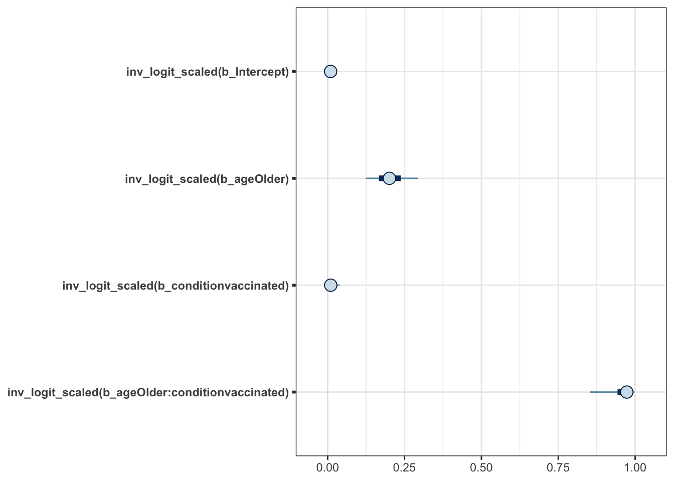

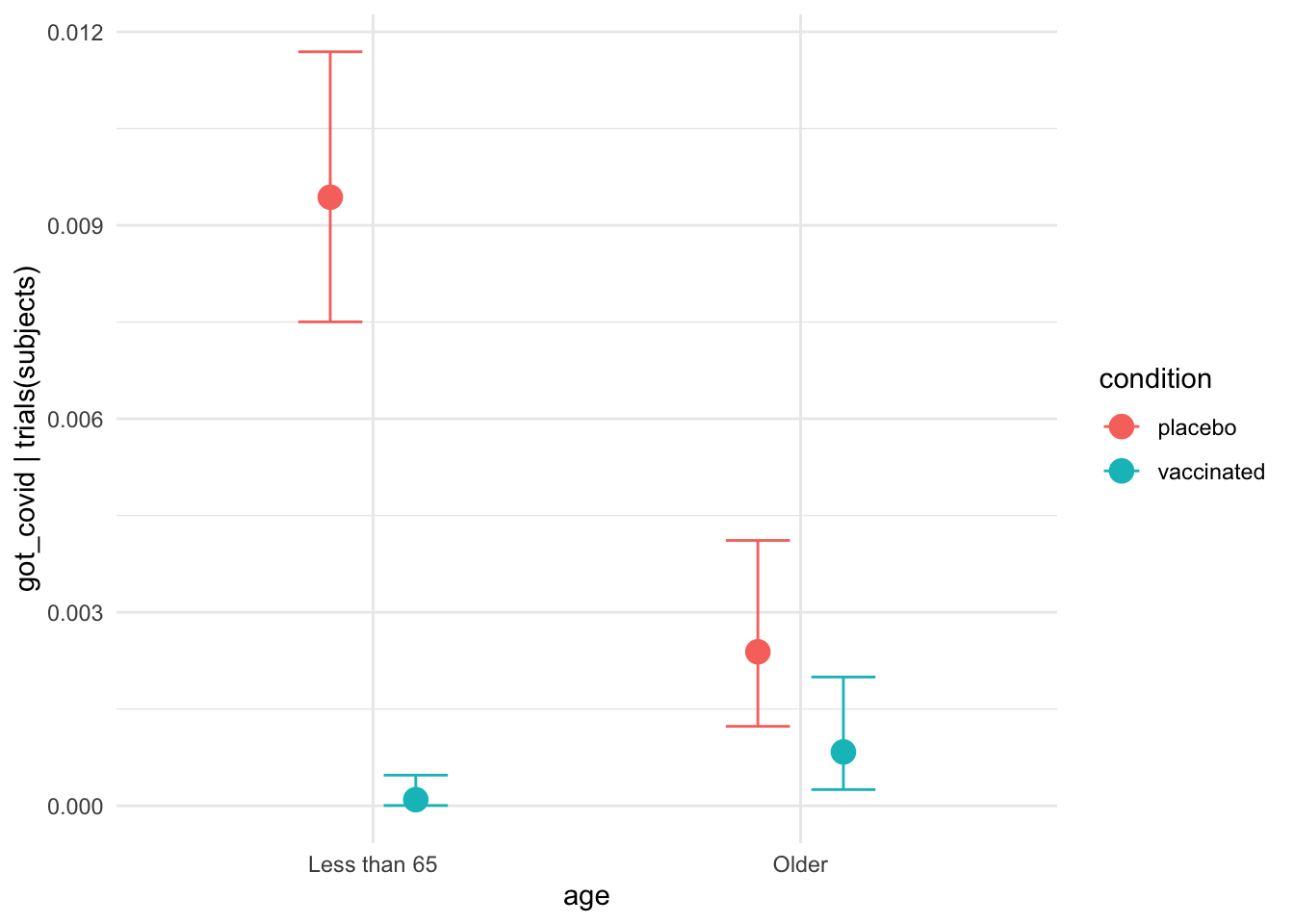
Honestly though \(\beta\) coefficients are sometimes hard to explain to someone not familiar with the regression framework. Let’s talk about conditional effects. brms provides a handy functional called conditional_effects that will plot them for us. The command conditional_effects(moderna_bayes_full) is enough to get us a decent output, but we can also wrap it in plot and do things like change the ggplot theme. We can focus on just the interaction effect with effects = "age:condition". This is important because interpreting main effects when we have evidence of an interaction is dubious. We can even pass additional ggplot information to customize our plot.

# conditional_effects(moderna_bayes_full)

plot(conditional_effects(moderna_bayes_full), 
     theme = ggplot2::theme_minimal())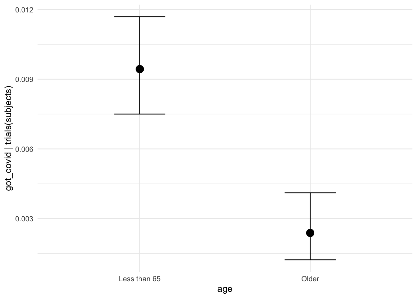

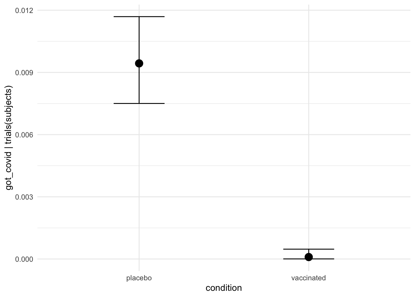
interaction_effect <-
   plot(conditional_effects(moderna_bayes_full,
                            effects = "age:condition",
                            plot = FALSE), 
        theme = ggplot2::theme_minimal())

interaction_effect$`age:condition`  +
   ggplot2::ggtitle("Infection rate by condition") +
   ggplot2::ylab("Infected / Subjects per condition") +
   ggplot2::xlab("Age") +
   ggplot2::theme_minimal()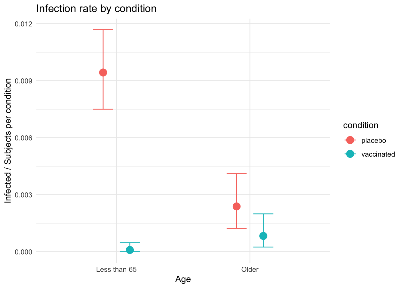

If this data were real it would give us pause since it highlights the fact that the vaccine appears to be much less effective for people over the age of 65.

If you don’t like the appearance of the plots from brms or prefer making use of bayestestR as we did in earlier posts it is trivial to extract the draws/chains and plot it.

# library(bayestestR)
moderna_draws <- 
   tidybayes::tidy_draws(moderna_bayes_full) %>%
   select(b_Intercept:`b_ageOlder:conditionvaccinated`) %>%
   mutate_all(inv_logit_scaled)

moderna_draws

## # A tibble: 48,000 x 4
##    b_Intercept b_ageOlder b_conditionvaccinated `b_ageOlder:conditionvaccinated`
##          <dbl>      <dbl>                 <dbl>                            <dbl>
##  1     0.00827      0.351               0.0160                             0.948
##  2     0.00954      0.164               0.0110                             0.958
##  3     0.00955      0.242               0.0202                             0.962
##  4     0.00876      0.240               0.0176                             0.896
##  5     0.00999      0.157               0.00496                            0.981
##  6     0.0129       0.171               0.00266                            0.994
##  7     0.00919      0.181               0.00442                            0.993
##  8     0.00971      0.244               0.0259                             0.937
##  9     0.00900      0.147               0.00749                            0.982
## 10     0.00893      0.172               0.00975                            0.977
## # … with 47,990 more rows

plot(bayestestR::hdi(moderna_draws, ci = c(.89, .95)))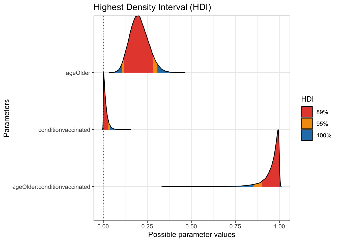

Priors and Bayes Factors

Bayesian analysis rests on the principle of modeling how the data inform our prior beliefs about understanding. You’ll notice that no where above did I specify any prior. That’s because brms is kind enough to provide defaults. From the documentation “Default priors are chosen to be non or very weakly informative so that their influence on the results will be negligible and you usually don’t have to worry about them. However, after getting more familiar with Bayesian statistics, I recommend you to start thinking about reasonable informative priors for your model parameters: Nearly always, there is at least some prior information available that can be used to improve your inference.”

To be conservative but also to pave the way for computing some Bayes Factors let’s consult the STAN documentation and some weakly informative priors. We can run get_prior to get back information about the defaults. We don’t really care about the overall intercept \(\beta_0\) but let’s set the others to normal(0,3) which puts us between weak and very weak. We’ll store those changes in bprior, rerun the model with a new name and you can see that changing the priors to something slightly more informative has little impact. The data overwhelms the priors and our posteriors are about the same as they were.

get_prior(data = agg_moderna_data,
       family = binomial(link = logit),
       got_covid | trials(subjects) ~ age + condition + age:condition)

##                 prior     class                         coef group resp dpar
##                (flat)         b                                             
##                (flat)         b                     ageOlder                
##                (flat)         b ageOlder:conditionvaccinated                
##                (flat)         b          conditionvaccinated                
##  student_t(3, 0, 2.5) Intercept                                             
##  nlpar bound       source
##                   default
##              (vectorized)
##              (vectorized)
##              (vectorized)
##                   default

### https://github.com/stan-dev/stan/wiki/Prior-Choice-Recommendations
### Generic weakly informative prior: normal(0, 1);
bprior <- c(prior(normal(0,3), class = b, coef = ageOlder),
            prior(normal(0,3), class = b, coef = conditionvaccinated),
            prior(normal(0,3), class = b, coef = ageOlder:conditionvaccinated))
bprior

##         prior class                         coef group resp dpar nlpar bound
##  normal(0, 3)     b                     ageOlder                            
##  normal(0, 3)     b          conditionvaccinated                            
##  normal(0, 3)     b ageOlder:conditionvaccinated                            
##  source
##    user
##    user
##    user

full_model <-
   brm(data = agg_moderna_data,
       family = binomial(link = logit),
       got_covid | trials(subjects) ~ age + condition + age:condition,
       prior = bprior,
       iter = 12500,
       warmup = 500,
       chains = 4,
       cores = 4,
       seed = 9,
       save_pars = save_pars(all = TRUE),
       file = "full_model")
summary(full_model)

##  Family: binomial 
##   Links: mu = logit 
## Formula: got_covid | trials(subjects) ~ age + condition + age:condition 
##    Data: agg_moderna_data (Number of observations: 4) 
## Samples: 4 chains, each with iter = 12500; warmup = 500; thin = 1;
##          total post-warmup samples = 48000
## 
## Population-Level Effects: 
##                              Estimate Est.Error l-95% CI u-95% CI Rhat Bulk_ESS
## Intercept                       -4.67      0.11    -4.90    -4.45 1.00    49307
## ageOlder                        -1.33      0.32    -1.99    -0.74 1.00    29645
## conditionvaccinated             -3.97      0.76    -5.67    -2.69 1.00    15090
## ageOlder:conditionvaccinated     2.76      0.96     0.96     4.75 1.00    16749
##                              Tail_ESS
## Intercept                       38807
## ageOlder                        26856
## conditionvaccinated             15787
## ageOlder:conditionvaccinated    18968
## 
## Samples were drawn using sampling(NUTS). For each parameter, Bulk_ESS
## and Tail_ESS are effective sample size measures, and Rhat is the potential
## scale reduction factor on split chains (at convergence, Rhat = 1).

Some bayesians like to work with a Bayes Factor. We can use brms::bayes_factor to inform us about the relative worthiness of competing regression models. You’ll notice I named the first set of results full_model because it included age, condition and the interaction between them age:condition. Let’s build three more models:

• one without the interaction term called no_interaction,
• one without the interaction or the vaccine called no_vaccine,
• one without the interaction or age called no_age,

Then we can compare the full model against each of these nested models. (NB for the purists yes I actually tried some other priors that were less weak and yes the bayes factors are quite robust.)

bprior2 <- c(prior(normal(0,3), class = b, coef = ageOlder),
            prior(normal(0,3), class = b, coef = conditionvaccinated))
bprior2

##         prior class                coef group resp dpar nlpar bound source
##  normal(0, 3)     b            ageOlder                               user
##  normal(0, 3)     b conditionvaccinated                               user

no_interaction <-
   brm(data = agg_moderna_data,
       family = binomial(link = logit),
       got_covid | trials(subjects) ~ age + condition,
       prior = bprior2,
       iter = 12500,
       warmup = 500,
       chains = 4,
       cores = 4,
       seed = 9,
       save_pars = save_pars(all = TRUE),
       file = "no_interaction")
summary(no_interaction)

##  Family: binomial 
##   Links: mu = logit 
## Formula: got_covid | trials(subjects) ~ age + condition 
##    Data: agg_moderna_data (Number of observations: 4) 
## Samples: 4 chains, each with iter = 12500; warmup = 500; thin = 1;
##          total post-warmup samples = 48000
## 
## Population-Level Effects: 
##                     Estimate Est.Error l-95% CI u-95% CI Rhat Bulk_ESS Tail_ESS
## Intercept              -4.70      0.12    -4.94    -4.48 1.00    52909    38740
## ageOlder               -1.07      0.28    -1.65    -0.55 1.00    22774    21953
## conditionvaccinated    -2.87      0.45    -3.83    -2.08 1.00    18737    19745
## 
## Samples were drawn using sampling(NUTS). For each parameter, Bulk_ESS
## and Tail_ESS are effective sample size measures, and Rhat is the potential
## scale reduction factor on split chains (at convergence, Rhat = 1).

bprior3 <- c(prior(normal(0,3), class = b, coef = ageOlder))
bprior3

## b_ageOlder ~ normal(0, 3)

no_vaccine <-
   brm(data = agg_moderna_data,
       family = binomial(link = logit),
       got_covid | trials(subjects) ~ age,
       prior = bprior3,
       iter = 12500,
       warmup = 500,
       chains = 4,
       cores = 4,
       seed = 9,
       save_pars = save_pars(all = TRUE),
       file = "no_vaccine")
summary(no_vaccine)

##  Family: binomial 
##   Links: mu = logit 
## Formula: got_covid | trials(subjects) ~ age 
##    Data: agg_moderna_data (Number of observations: 4) 
## Samples: 4 chains, each with iter = 12500; warmup = 500; thin = 1;
##          total post-warmup samples = 48000
## 
## Population-Level Effects: 
##           Estimate Est.Error l-95% CI u-95% CI Rhat Bulk_ESS Tail_ESS
## Intercept    -5.34      0.11    -5.56    -5.12 1.00    48533    33484
## ageOlder     -1.07      0.28    -1.65    -0.54 1.00    16100    17671
## 
## Samples were drawn using sampling(NUTS). For each parameter, Bulk_ESS
## and Tail_ESS are effective sample size measures, and Rhat is the potential
## scale reduction factor on split chains (at convergence, Rhat = 1).

bprior4 <- c(prior(normal(0,3), class = b, coef = conditionvaccinated))
bprior4

## b_conditionvaccinated ~ normal(0, 3)

no_age <-
   brm(data = agg_moderna_data,
       family = binomial(link = logit),
       got_covid | trials(subjects) ~ condition,
       prior = bprior4,
       iter = 12500,
       warmup = 500,
       chains = 4,
       cores = 4,
       seed = 9,
       save_pars = save_pars(all = TRUE),
       file = "no_age")
summary(no_age)

##  Family: binomial 
##   Links: mu = logit 
## Formula: got_covid | trials(subjects) ~ condition 
##    Data: agg_moderna_data (Number of observations: 4) 
## Samples: 4 chains, each with iter = 12500; warmup = 500; thin = 1;
##          total post-warmup samples = 48000
## 
## Population-Level Effects: 
##                     Estimate Est.Error l-95% CI u-95% CI Rhat Bulk_ESS Tail_ESS
## Intercept              -4.96      0.11    -5.17    -4.76 1.00    52371    33818
## conditionvaccinated    -2.88      0.45    -3.85    -2.07 1.00    10390    11347
## 
## Samples were drawn using sampling(NUTS). For each parameter, Bulk_ESS
## and Tail_ESS are effective sample size measures, and Rhat is the potential
## scale reduction factor on split chains (at convergence, Rhat = 1).

bayes_factor(full_model, no_interaction, silent = TRUE)

## Estimated Bayes factor in favor of full_model over no_interaction: 31.06810

bayes_factor(full_model, no_vaccine, silent = TRUE)

## Estimated Bayes factor in favor of full_model over no_vaccine: 235611405759697158144.00000

bayes_factor(full_model, no_age, silent = TRUE)

## Estimated Bayes factor in favor of full_model over no_age: 17306.61482

We can now quantify how well our models “fit” the data compared to the nested models. The evidence for retaining the model with the interaction term included is about 30:1. The evidence for keeping age is about 17,000:1 and you don’t even want to think about dropping the vaccine condition.

I do not personally believe in any model that includes an interaction but not the main effect that accompanies it.