Warpspeed vaccine vindication and an homage -- Part 3
Yahoo (not the service provider), yippee, and all those other cries of joy. After my last couple of posts what appears this morning…
Earlier on Monday, pharmaceutical giant Pfizer and its partner BioNTech said their experimental vaccine was 90% effective in preventing COVID-19. It is the first of the vaccine attempts to reach the clinical milestone. … That news comes from an interim analysis of a study involving 43,538 volunteers, 42% of whom had “diverse backgrounds.” … The vaccine proved to be more than 90% effective in the first 94 subjects who were infected by the new coronavirus and developed at least one symptom, the companies said Monday. … While promising, this analysis alone does not provide enough information about the vaccine for Pfizer to ask the FDA for permission to distribute it. … The agency has informed manufacturers that it wants a minimum of two months of follow-up data from at least half of the volunteers. The FDA says the reason for that requirement is that most dangerous side effects from a vaccine occur within two months of getting the final injection. Pfizer says that data won’t be available until the third week in November.
I’ve spent the last two posts exploring vaccine effectiveness (N.B. I have no data on safety this is just about effectiveness), and what should appear this morning but more data (always a good thing). Leaving aside the good news for humanity it means my timing is great and I get to have more fun as well as following through on my plan to show a little respect for a great book.
In my last two posts I did some basic statistical analysis of how confident we should feel about the effectiveness of a vaccine for COVID-19 (Operation Warpspeed). A reminder I’m not an epidemiologist, I don’t have any data for safety, and we’re still quite early in the Phase III trials – just past the point at which they can take a first “peek” at the data (which is doubleblind). You’ll be best served if you’ve already read the previous post.
You can also read the full study design and justification online although it runs to 136 pages before references.
That’s where we’ll pick up in this post. First let’s load some essential libraries.
library(dplyr)
library(ggplot2)
library(kableExtra)
theme_set(theme_bw())
Last time
Last time we used a variety of bayesian tools and techniques to model our potential results. At the time we were looking at Moderna possibilities, as it turns out Pfizer got there first (the more successful candidates the better as far as I’m concerned).
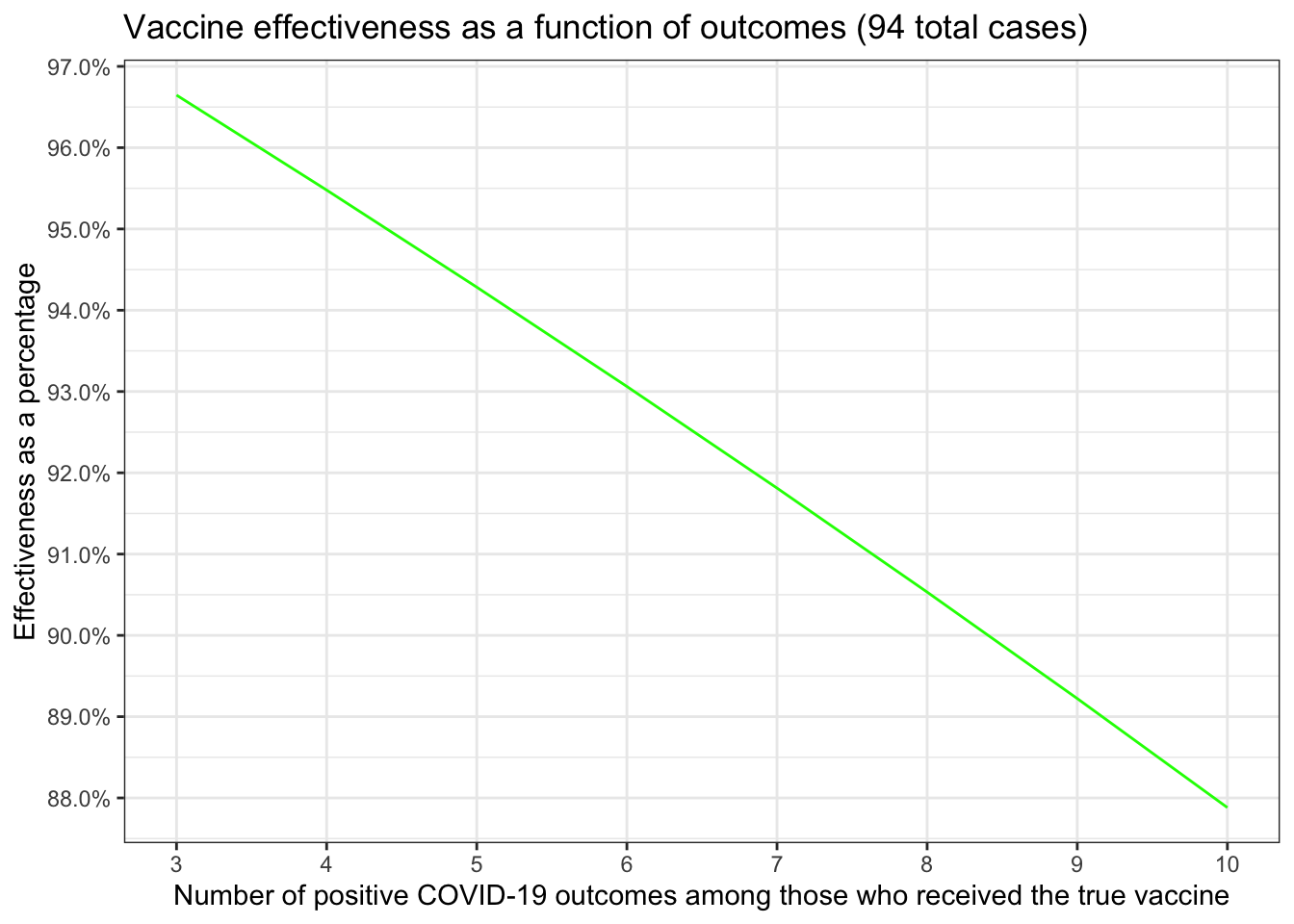
Since each of the trials is slightly different in terms of numbers let’s replicate the little table from the first post about effectiveness. That gave us estimates for the rate of infection for both those who received the placebo and those who received the actual vaccine. \[\frac{placebo~infection~rate - vaccinated~infection~rate}{placebo~infection~rate} \times 100\] This gives us what we really want to investigate which is the percentage difference in infection rates. We’re looking for (since we multiplied by 100) a number that is above 90. Here’s the little table and chart we made in the first post updated for the Pfizer data.
|
Covid Cases (94)
|
Infection Rate
|
% difference in rate
|
||
|---|---|---|---|---|
| vaccinated | placebo | placeborate | vaccinatedrate | effectiveness |
| 3 | 91 | 0.0042 | 0.00014 | 96.65 |
| 4 | 90 | 0.0041 | 0.00019 | 95.48 |
| 5 | 89 | 0.0041 | 0.00023 | 94.28 |
| 6 | 88 | 0.0040 | 0.00028 | 93.06 |
| 7 | 87 | 0.0040 | 0.00033 | 91.81 |
| 8 | 86 | 0.0039 | 0.00037 | 90.53 |
| 9 | 85 | 0.0039 | 0.00042 | 89.22 |
| 10 | 84 | 0.0038 | 0.00046 | 87.88 |
Okay now that you’re caught up let’s push our bayesian skills even farther.
Last post
we used several different tools to explore our confidence and the credibility
of the data. We used bayesAB, ggdist, bayestestR, brms, tidybayes
and STAN to name more than a few. They all produced comparable results which
echoed our initial homespun foray from the first post.
Today we’re going to use the new Pfizer data and take one more look while paying homage to Doing Bayesian Data Analysis by Dr. John K. Kruschke. Hereafter, simply DBDA. It’s a classic and was my first academic foray into the topic. As opposed to just using tools in R. There are newer books and newer tools but it really does stand the test of time. Having been effusive in my praise which is well deserved I must confess that from the perspective of R code and tools it feels a bit quaint. It was written to make sure that it worked well on a variety of platforms in a much earlier time for beginners. A spectacular feat. But I want to explore the topic with less code and more modern tools.
In chapter 8 (8.4 – EXAMPLE: DIFFERENCE OF BIASES) Kruschke explores an example
of the differences between two coins using R. Actually, he starts the example in
7.4 with an eerily on point example of a drug trial! In today’s post we’re
going to simply adapt the code and modrnize it a bit with some more current
R tools to use on our warpspeed trials.
The original DBDA code envisions our Pfizer data as a long dataframe with
two columns. One column has information about whether or not the
participant tested positive for COVID-19 the other column has
information about whether they received the “true” vaccine or a placebo.
It’s 43,538 rows, 21,999 of whom received the “true” vaccine stored
in column s, column y has Yes or No as a character vector for
whether they tested positive for COVID-19. This is where our split
is 8 & 86 for the 94 cases. We’ll take a glimpse and build a
quick table to make sure we got it right.
pfizer_data <-
   data.frame(
      y = c(rep("No", 21999 - 8),
            rep("Yes", 8),
            rep("No", 21539 - 86),
            rep("Yes", 86)),
      s = c(rep("vaccinated", 21999),
            rep("placebo", 21539))
      )

glimpse(pfizer_data)
## Rows: 43,538
## Columns: 2
## $ y <chr> "No", "No", "No", "No", "No", "No", "No", "No", "No", "No", "No", "…
## $ s <chr> "vaccinated", "vaccinated", "vaccinated", "vaccinated", "vaccinated…table(pfizer_data$s, pfizer_data$y)##
## No Yes
## placebo 21453 86
## vaccinated 21991 8In my earlier posts I have been using a flat uninformed prior. That’s
not “bad” since in bayesian inference an abundance of data, as we have,
will overcome (correct/update) the priors even if they are off, that’s
the point. But just to be a little more accurate let’s pick priors
that are more like our beliefs. Remember that these priors are
not about our belief in how effective the vaccine is, rather they
are about our prior knowledge of how likely it is to get COVID-19 in
either condition \(\theta[1]\) and \(\theta[2]\). We could express
different values for each but we won’t. We just want a prior that
expresses our knowledge that for both of them infection rates are very
low – whether they received the placebo or the true vaccine the
likelihood of contracting COVID-19 appears to be less than 1%. Using
bayesAB::plotBeta(3, 100) to plot it something like this.
bayesAB::plotBeta(3, 100)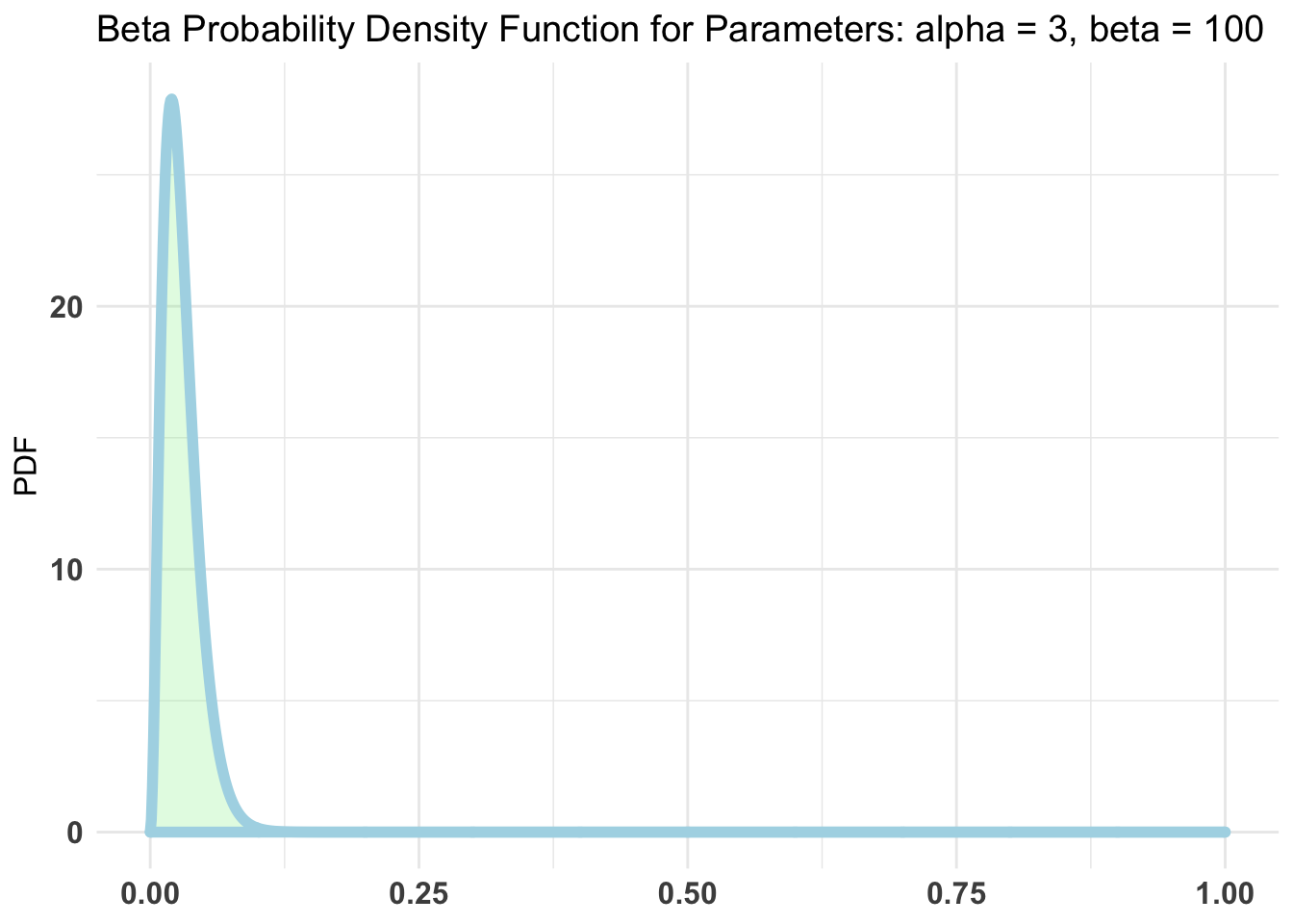
We’re treating COVID-19 outcomes as simple binomial equations (a coin flip if
you will). But both of our coins are unlikely to have equal numbers of
positive versus negative cases. That leads us to expressing our model in the
JAGS language before we feed it to run.jags. To simply quote from DBDA
In the above code, notice that the index i goes through the total number of data values, which is the total number of rows in the data file. So you can also think of i as the row number. The important novelty of this model specification is the use of “nested indexing” for theta[s[i]] in the dbern distribution. For example, consider when the for loop gets to i = 12. Notice from the data file that s[12] is 2. Therefore, the statement y[i] ∼ dbern(theta[s[i]]) becomes y[12] ∼ dbern(theta[s[12]]) which becomes y[12] ∼ dbern(theta[2]). Thus, the data values for subject s are modeled by the appropriate corresponding θs.
# THE MODEL.
modelString <- "
  model {
    for ( i in 1:Ntotal ) {
      y[i] ~ dbern( theta[s[i]] )
    }
    for ( sIdx in 1:Nsubj ) {
      theta[sIdx] ~ dbeta(3 , 100)
    }
  }
  " # close quote for modelString
So we have a dataframe with our Pfizer data, priors, and a model. What we
need to do now is make sure the data is in a format run.jags can understand
and express any preferences we have for starting values for our chains. The data
is pretty straight-forward and hopefully a little clearer than the way
DBDA approaches it. Our model tells us we need 4 data elements, y, s,
Ntotal, and Nsubj. Let’s get these right from pfizer_data on the
fly. We know that pfizer_data$y is either character or factor so
a simple ifelse gets us to the 0/1 format we need. s also needs to be
numeric but an integer starting at 1 for however many categories there
are so we’ll force to factor and then integer. Ntotal is simply the
total number of particpants nrow and Nsubj the number of
categories for s. Voila.
# Specify the data in a list, for later shipment to JAGS:
dataList = list(
   y = ifelse(pfizer_data$y == "No", 0, 1),
   s = as.integer(factor(pfizer_data$s)),
   Ntotal = nrow(pfizer_data) ,
   Nsubj = nlevels(factor(pfizer_data$s))
)
runjags::run.jags is actually very good about setting initial
values but for the practice we’ll develop our own little function. The
doco says “or a function with either 1 argument representing the chain
or no arguments.” Since we plan on running it in parallel we’ll
make use of the chain parameter. The doco states “The special variables
‘.RNG.seed’, ‘.RNG.name’, and ‘.RNG.state’ are allowed for explicit control
over random number generators in JAGS.” Again, the default behavior is
perfectly fine but while we’re playing we may as well. So for
our random number generation we’ll use base::Super-Duper. To generate
reasonable distinct initial \(\theta[1]\) and \(\theta[2]\) values for
each parallel process we’ll use a small for loop and sample the
actual data. The 0.001 + 0.998 * sum(resampledy) / length(resampledy)
code is an idea from DBDA to keep us from accidentally going to
zero. We test it against a notional chain = 3.
initsfunctionX <- function(chain) {
   .RNG.seed <- c(1:chain)[chain]
   .RNG.name <- rep("base::Super-Duper", chain)[chain]
   theta <- rep(sum(dataList$y) / length(dataList$y), dataList$Nsubj)
   for (i in min(dataList$s):max(dataList$s)) {
      resampledy <- sample(dataList$y[dataList$s == i], replace=TRUE )
      theta[i] <- 0.001 + 0.998 * sum(resampledy) / length(resampledy)
   }

   return(list(.RNG.seed = .RNG.seed,
               .RNG.name = .RNG.name,
               theta = theta))
}

initsfunctionX(3)
## $.RNG.seed
## [1] 3
##
## $.RNG.name
## [1] "base::Super-Duper"
##
## $theta
## [1] 0.005262779 0.001226828Okay now we have all the requisite pieces let’s roll. 4 chains in parallel each sampling 15,000 with the default burnin = 4000. The chains converge nicely. No problems with auto-correlation or cross correlation.
pfizer_chains <-
   runjags::run.jags(modelString,
                     sample = 15000,
                     n.chains = 4,
                     method = "parallel",
                     monitor = "theta",
                     data = dataList,
                     inits = initsfunctionX)
## Calling 4 simulations using the parallel method...
## Following the progress of chain 1 (the program will wait for all chains
## to finish before continuing):
## Welcome to JAGS 4.3.0 on Tue Nov 10 15:24:57 2020
## JAGS is free software and comes with ABSOLUTELY NO WARRANTY
## Loading module: basemod: ok
## Loading module: bugs: ok
## . . Reading data file data.txt
## . Compiling model graph
## Resolving undeclared variables
## Allocating nodes
## Graph information:
## Observed stochastic nodes: 43538
## Unobserved stochastic nodes: 2
## Total graph size: 87082
## . Reading parameter file inits1.txt
## . Initializing model
## . Adaptation skipped: model is not in adaptive mode.
## . Updating 4000
## -------------------------------------------------| 4000
## ************************************************** 100%
## . . Updating 15000
## -------------------------------------------------| 15000
## ************************************************** 100%
## . . . . Updating 0
## . Deleting model
## All chains have finished
## Note: the model did not require adaptation
## Simulation complete. Reading coda files...
## Coda files loaded successfully
## Calculating summary statistics...
## Calculating the Gelman-Rubin statistic for 2 variables....
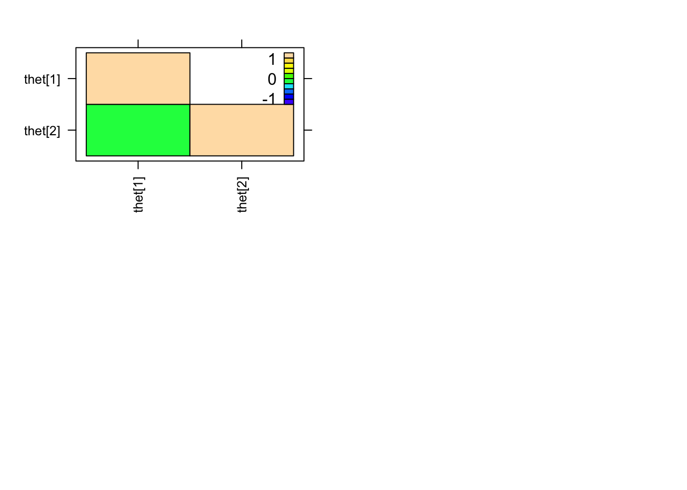
## Finished running the simulationsummary(pfizer_chains)## Lower95 Median Upper95 Mean SD Mode
## theta[1] 0.003266840 0.0041005650 0.004955990 0.0041170315 0.0004329743 NA
## theta[2] 0.000227758 0.0004830805 0.000801565 0.0004981343 0.0001504770 NA
## MCerr MC%ofSD SSeff AC.10 psrf
## theta[1] 2.168746e-06 0.5 39857 -0.0001435265 1.000007
## theta[2] 7.432855e-07 0.5 40985 0.0006641947 1.000047plot(pfizer_chains)## Generating plots...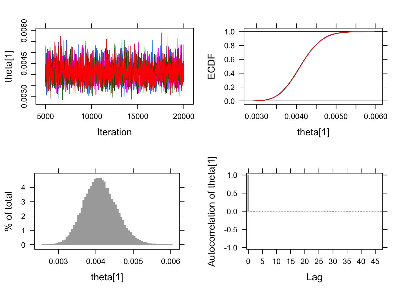
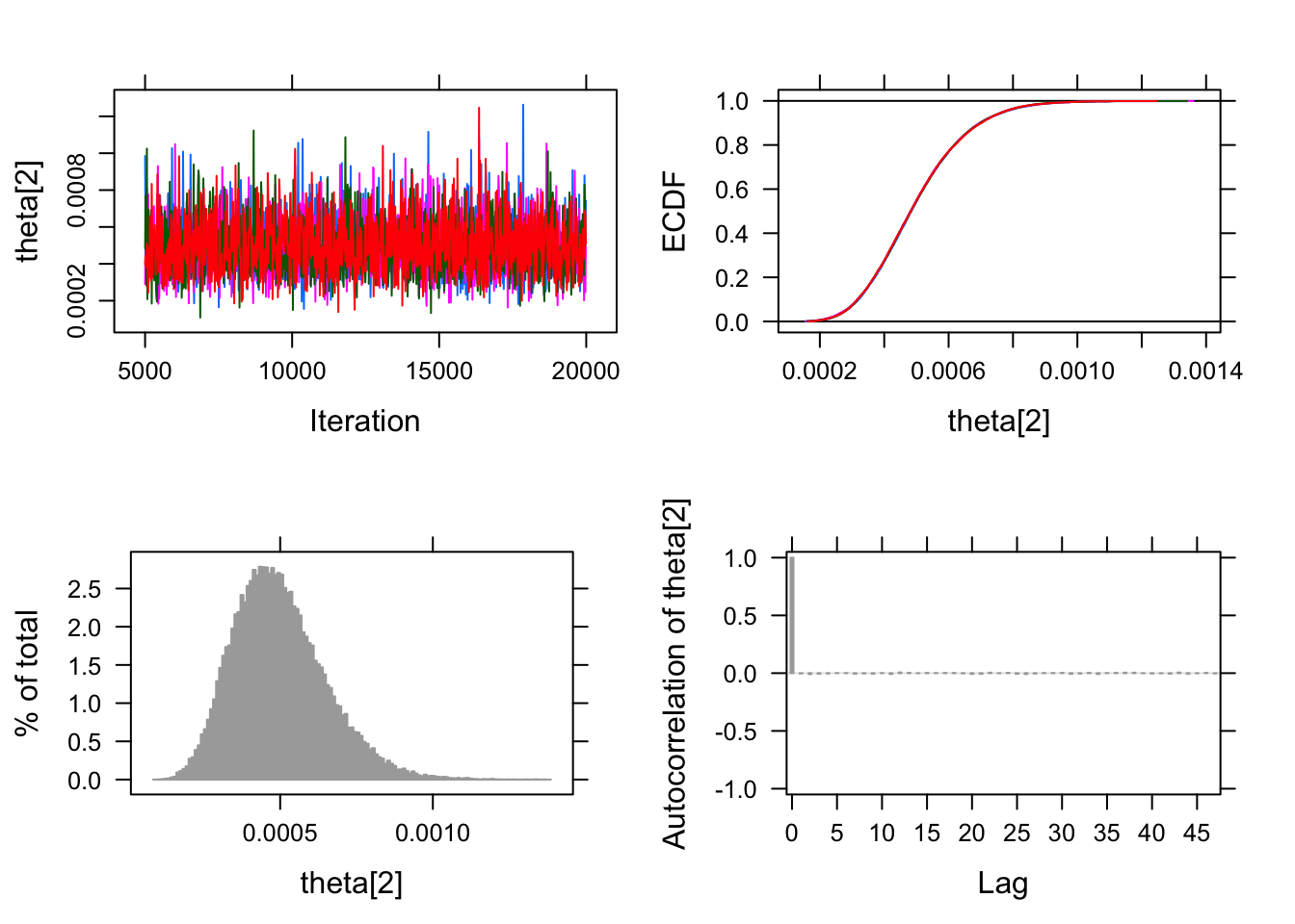
As usual this gives us estimates for the rate of infection for both
those who received the placebo and those who received the actual vaccine.
We can use tidybayes::tidy_draws to extract the chains/draws. We’re not
really interested in tracking the .chain, .iteration, and .draw
information so we’ll select just the two \(\theta\)s we’re interested
in. Since Greek letters are sometimes hard to follow we’ll
rename them back to placebo and vaccinated and multiply by 100 to
give us percent as in 8/21999 * 100 = 0.03% infection rate for
those that received the true vaccine.
Then we calculate what we really want to investigate which is the percentage
difference in infection rates. We’re looking for (since we multiplied by 100) a
number that is around 90. Which in essence is a 90% effectiveness rating. A
series of calls to bayestestR::hdi gives us graphical portrayals of what we want
to know. We see that more 99% of our draws wind up with a solution greater than
75% effective. That gives us great credibility or confidence that given our data
the effectiveness is there.
library(bayestestR)
pfizer_results <-
   tidybayes::tidy_draws(pfizer_chains) %>%
   select(`theta[1]`:`theta[2]`) %>%
   rename(placebo = `theta[1]`, vaccinated = `theta[2]`) %>%
   mutate(diff_rate = (placebo - vaccinated) / placebo * 100,
          placebo_pct = placebo * 100,
          vaccinated_pct = vaccinated * 100)

plot(bayestestR::hdi(pfizer_results$placebo_pct))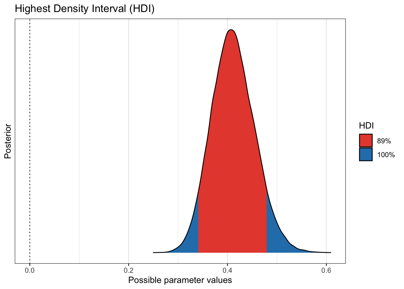
plot(bayestestR::hdi(pfizer_results$vaccinated_pct))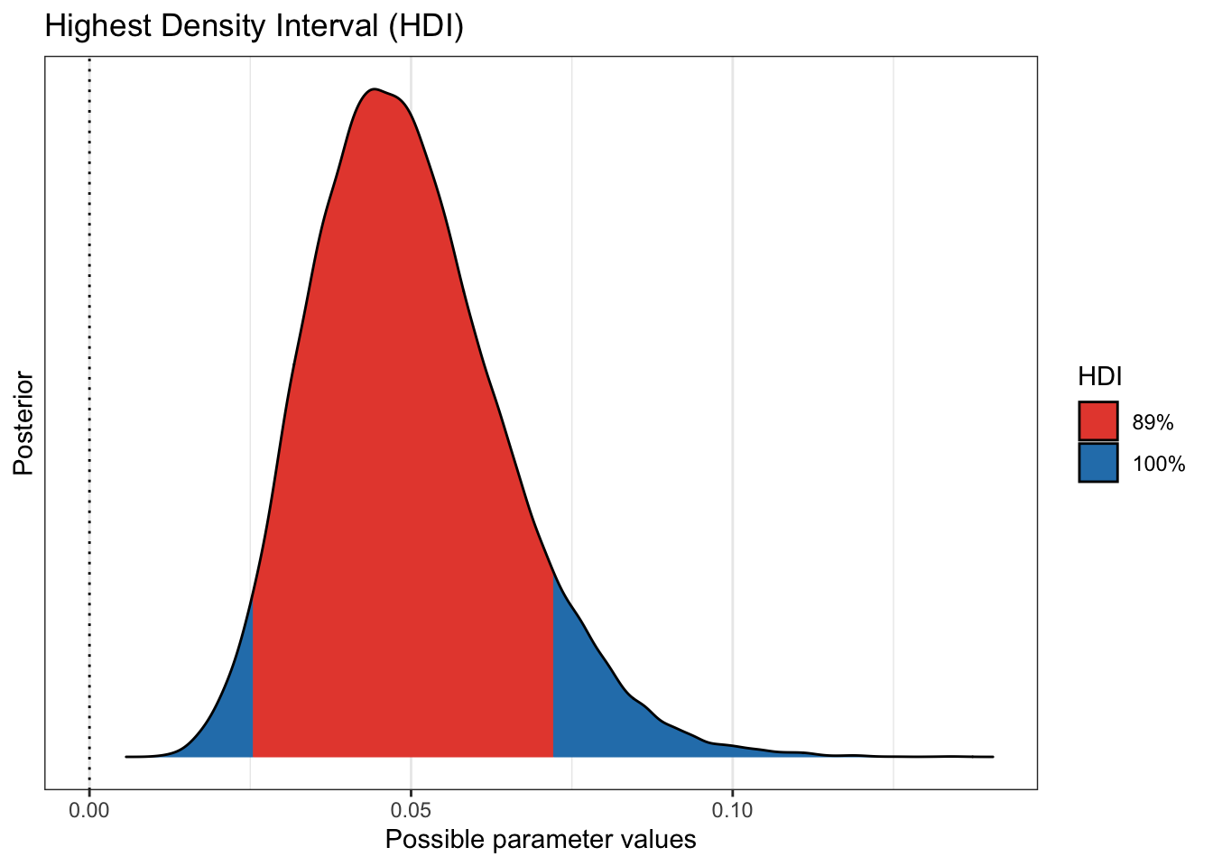
plot(bayestestR::hdi(pfizer_results$diff_rate, ci = c(.89, .95, .99)))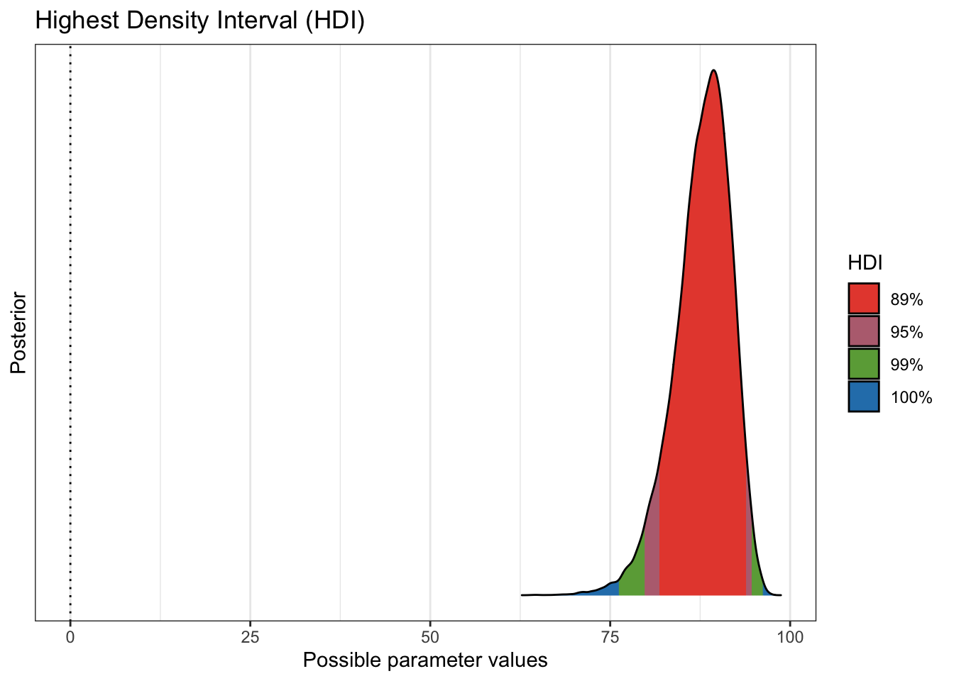
plot(bayestestR::point_estimate(pfizer_results$diff_rate))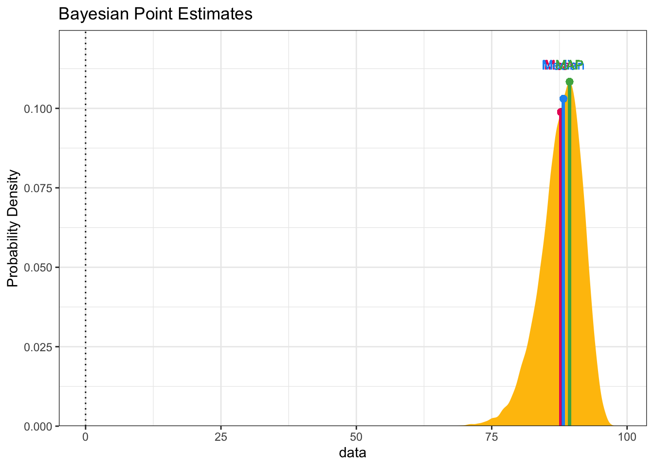
More credibility for our results
Bayesian don’t usually like to talk about significance, but we can show similar concepts with ROPE and practical significance (PS).
plot(bayestestR::rope(pfizer_results$diff_rate, range = c(0, 50)))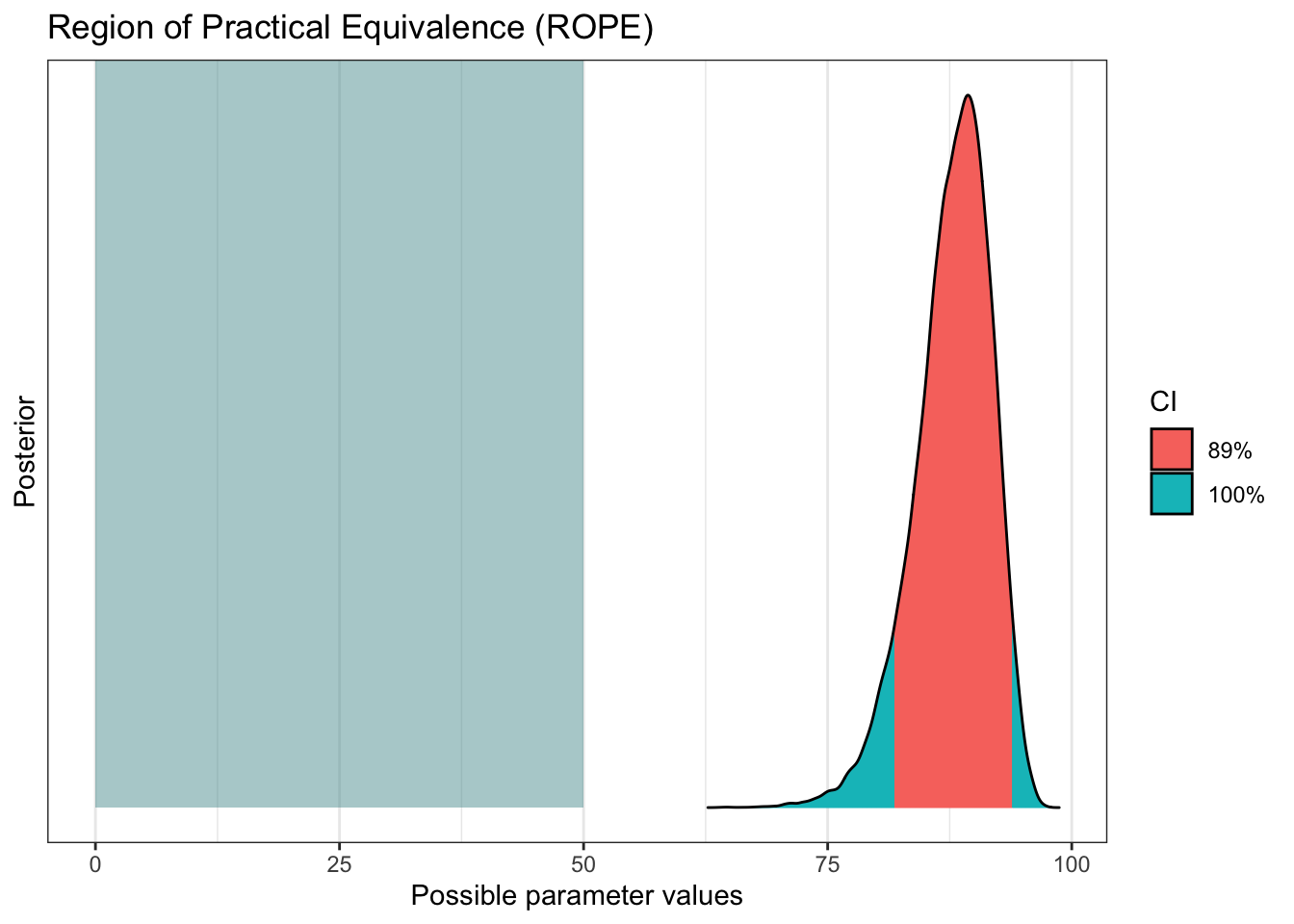
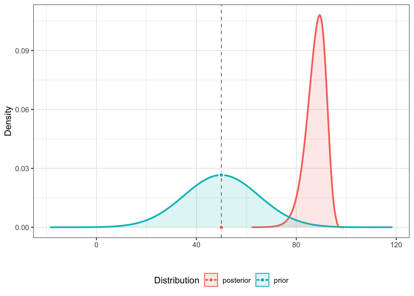
bayestestR::p_significance(pfizer_results$diff_rate, threshold = 50)## ps [50.00] = 100.00%bayestestR::p_significance(pfizer_results$diff_rate, threshold = 75)## ps [75.00] = 99.43%bayestestR::p_significance(pfizer_results$diff_rate, threshold = 90)## ps [90.00] = 31.09%Some bayesians like to work with a Bayes Factor. There’s even a fantastic
r package named BayesFactor that focuses on them. A quick example is
in order. Suppose that our prior belief before seeing the data was
that the Pfizer vaccine would be 50% effective but with a standard
deviation of 15% around that 50%. We can operationalize that simply with
prior <- distribution_normal(60000, mean = 50, sd = 15). Then we can use
bayesfactor_parameters(pfizer_results$diff_rate, prior, direction = "two-sided", null = 50)
to compute the odds that with our priors and our posteriors what are the
odds that the vaccine is more than 50% effective (two tailed to be conservative).
The answer is the odds given are data are more than 400,000:1 that the vaccine
is more than 50% effective. Overwhelming evidence.
prior <- distribution_normal(60000, mean = 50, sd = 15)
bayesfactor_parameters(pfizer_results$diff_rate, prior, direction = "two-sided", null = 50)
## Loading required namespace: logspline## # Bayes Factor (Savage-Dickey density ratio)
##
## BF
## ---------
## 4.159e+05
##
## * Evidence Against The Null: [50]plot(bayesfactor_parameters(pfizer_results$diff_rate, prior, direction = "two-sided", null = 50)
)
For extra credit don’t forget from my earlier posts that if you want the
ultimate in custom control over your plots ggdist can be your ally.
ggdist has a variety of nice functions
for summarizing and displaying draws and chains. stat_halfeye not only
plots it as a density curve but allows us to add per group credible intervals.
A “quick” example.
pfizer_results %>%
   select(placebo_pct:vaccinated_pct) %>%
   tidyr::pivot_longer(everything(), names_to = "group") %>%
   ggplot(aes(x = value, fill = group)) +
   ggdist::stat_halfeye(.width = c(0.89, 0.95),
                        alpha = .8,
                        slab_colour = "black",
                        slab_size = .5) +
   ggtitle("Infection rates for vaccine and placebo groups (N = 43,538)") +
   xlab("Infection rate") +
   scale_x_continuous(labels = scales::label_percent(scale = 1),
                      breaks = seq.int(0, .6, .1)) +
   theme(axis.title.y = element_blank(),
        axis.text.y = element_blank(),
        axis.ticks.y = element_blank(),
        panel.grid.major.y = element_blank(),
        panel.grid.minor.y = element_blank())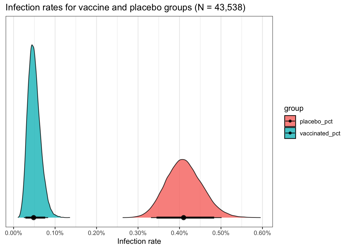
What have we learned?
The Pfizer vaccine appears to be tremendously effective. Let’s hope that the safety data is equally good. There will be a lot more analysis needed on a variety of factors like age, race, and gender as data accumulates.
DBDA is a timeless resource full of great information for data scientists and statisticians. But there are a lot faster and more elegant ways to code in
rthese days. Hopefully I’ve shown you a few while still honoring the book.
Done
I’m done with this topic for now. Fantastic news for humanity in the race for a vaccine.
Hope you enjoyed the post. Comments always welcomed. Especially please let me know if you actually use the tools and find them useful.
Keep counting the votes! Every last one of them!
Chuck

This work is licensed under a Creative Commons Attribution-ShareAlike 4.0 International License