Warspeed 5 -- priors and models continued
My last 4 posts have all focused on the
vaccines being produced to fight COVID-19. They have primarily focused on
Bayesian methods (or at least comparing bayesian to frequentist methods). This
one follows that pattern and provides expanded coverage of the concept of
priors in bayesian thinking, how to operationalize them, and additional
coverage of how to compare bayesian regression models using various tools in
r.
There’s no actual additional analysis of “real data”. While the news has all been good lately I haven’t found anything publicly available that begs for investigation. Instead we’ll use “realistic” but not real data, and let the process unfold for us.
I will, however, try to show you some tools and tricks in r to make your
analysis of any data easier and smoother.
What bayesians do
First off let me remind the reader that like most I was educated and trained in the frequentist tradition. I’m not against frequentist methods and even admit in the vast majority of cases they lead to similar conclusions. But, I do believe the bayesian methods are better and let you answer questions you really want to research. Now a quote from a great book, which also happens to be available at no cost.
From a Bayesian perspective, statistical inference is all about belief revision. I start out with a set of candidate hypotheses about the world. I don’t know which of these hypotheses is true, but do I have some beliefs about which hypotheses are plausible and which are not. When I observe the data, I have to revise those beliefs. If the data are consistent with a hypothesis, my belief in that hypothesis is strengthened. If the data is inconsistent with the hypothesis, my belief in that hypothesis is weakened. Navarro, page 555.
As a formula you’ll see Bayes Theorem expressed something like this:
\[P(hypothesis | data) = \frac{P(data | hypothesis) * P(hypothesis) }{P(data)}\]
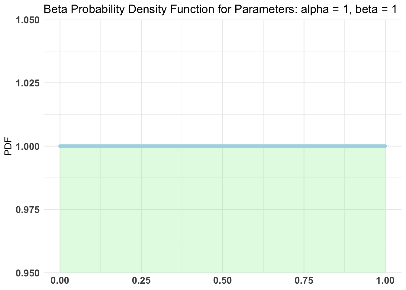
We have data, and we have hypotheses, we have bayesian tools, most “new” bayesians seem to stumble in the process of making good on our declaration of what our priors are. Up until today’s post I’ve mainly avoided the topic or briefly touched on and used terms like “vague”, “uninformed” or “flat”. See for example the very flat and uninformed plot from my second blog post in the series.
It’s okay in a bayesian framework to have priors that are vague if that’s what you really know and what you really mean. Just don’t use them when you know “more” or “better”. There is a real difference “between this value can be literally anything” and “this value we are studying has some prior knowledge behind it and some likely spread of values”.
And, no, you are absolutely NOT guaranteeing success or dooming failure if you are off on your priors. Obviously, as a scientist, you should pick values that make sense and not pluck them from thin air or make them up, but rest assured given sufficient data even priors that are “off” are adjusted by the data. Isn’t that the point after all? Develop a hypothesis and test it with data? Notice that in bayesian inference we don’t need to force a “null hypothesis” that we “reject”.
Come let us reason together
At this point if you’re not comfortable with bayesian inference I probably haven’t helped you at all and it all probably feels a bit theoretical. Let’s take our current vaccine problem and work it through.
Step 1 (what do we think we know or believe) about the vaccine and COVID-19
A vast amount of time, money, and science have gone into developing these vaccines, and in many cases they are products of years of previous research – if not about COVID-19 then at least other viruses. The candidate vaccines have already been tried in Phase I and Phase II in perhaps animals or in limited numbers of humans. They got to phase III not by being unknown or “anything is possible” but rather on a belief they are going to be at least 50% effective. So we know something about the direction and with less certainty something about the magnitude.
We know given public data that older people tend to contract COVID-19 less. All the data points to much higher infection rates in younger populations. Good thing too since the older population tends to have much more severe outcomes. Notice neither #1 or #2 says anything about how effective the vaccine is in older populations, we’ll get to that in a minute. But we certainly have evidence that currently older folks are less likely to get it. Notice reasonable people can disagree. It’s okay if you have scientific prior evidence that makes you think otherwise. Express it! Let the data inform us.
There is evidence that vaccines can be less effective for older populations. It is certainly a worry for scientists going into the trial. Just as there are worries for other health risk factors and potentially race and ethnicity and even gender as well. Chuck’s hypothesis is that the vaccine will be slightly less effective for older folks. But I’m prepared to be wrong and believe this less firmly than I believe the vaccine is effective.
Step 2 How do we make use of our prior knowledge?
In the last post
we used brms to build a bayesian equivalent of a glm model. That’s our plan
again today. So how do we go from my theoretical hypotheses in 1-3 above to
something we can feed into r and let it chew on and inform us with our data?
This is often the hard part for newcomers to bayesian inference. But it really
needn’t be if you focus on the basics. Our plan is to feed our hypotheses into a
generalized linear model. As with a the simpler case of modeling with lm we’ll
produce a model that gives us slope estimates (the venerable \(\beta\) or
\(\hat{b}_n\) coefficients). In traditional frequentist output these are in turn
tested against the hypothesis that they are zero and a pvalue is generated. Zero
slope means that predictor has zero ability to help us predict outcome in
\(y = \hat{b}_1 + \hat{b}_0\) if \(\hat{b}_1 = 0\) then \(y = \hat{b}_0\) the intercept and
\(\hat{b}_1\) can be eliminated.
So our priors need to be converted to something that makes sense as a value for \(\hat{b}_n\). No effect equals zero and bigger effects mean larger positive or negative values. Notice that our estimates have a standard error which means they have a standard deviation which will serve as a way of expressing our “confidence” about our priors. A small value means we’re more sure that the effect will be tightly centered, larger SD means we’re less certain.
So going back to 1-3 above let’s proceed with our priors one by one.
Vaccine effect – So we know something about the direction and with less certainty something about the magnitude. We could pick from a large number of possible distributions for our \(\hat{b}_n\) here but hopefully you’re thinking by now this sounds like a
normalortdistribution with an appropriatesdandmean. With small amounts of datatis possibly a better choice, but remember our data will inform us we are NOT fixing the outcome. So let’s set a prior for \(\hat{b}_{conditionvaccinated}\) with the mean at -2.0 and the sd of .5. Why a minus sign? That’s because \(\hat{b}_{conditionvaccinated}\) compares to the placebo condition and therefore the number of people who got COVID-19 in the trial will be less. The .5 sd is because we think the vaccine will be at least moderately effective. No worries later I’ll show you how to be more specific in your hypotheses. You’ll see this later but forbrmsandSTANwe express this asprior(normal(-2.0, .5), class = b, coef = conditionvaccinated)Older folks are less likely to get COVID-19. Remember this is a general statement about older folks regardless of whether they received the placebo or the vaccine. This difference is less pronounced and less certain so we’ll set the mean closer to zero at -.5 and increase the standard deviation to 1 to indicate we believe it’s more variable and that is expressed as
prior(normal(-0.5, 1), class = b, coef = ageOlder).Chuck’s hypothesis is that the vaccine will be slightly less effective for older folks. Which means that this time the sign will be positive because the interaction
ageOlder:conditionvaccinatedwill yield slightly higher infection rates and therefore \(\hat{b}_{ageOlder:conditionvaccinated}\) will be a small positive number. But I’m less firm in this belief so once again standard deviation = 1 and the code isprior(normal(.5, 1), class = b, coef = ageOlder:conditionvaccinated)
Now, we have reasonable informed priors! And hopefully you have a better idea
on how to set them in a regression model of interest to you. Remember you
can consult the STAN documentation
for more suggestions on informative priors. We can run get_prior to get back
information about the defaults. Notice we don’t really care about the overall
intercept \(\hat{b}_0\).
Load libraries and on to the data
Load the necessary libraries as before
library(dplyr)
library(brms)
library(ggplot2)
library(kableExtra)
theme_set(theme_bw())
Load the same data as last time, this time I’m providing it as a
structure for your ease. Again you could have your data in full
long format and accomplish the same modeling I’m providing it
wide and summarized for computational speed and leaving you the dplyr
commands to go long if you like.
agg_moderna_data <-
   structure(list(
      condition = structure(c(1L, 1L, 2L, 2L), .Label = c("placebo", "vaccinated"), class = "factor"),
      age = structure(c(1L, 2L, 1L, 2L), .Label = c("Less than 65", "Older"), class = "factor"),
      didnot = c(9900L, 993L, 9990L, 999L),
      got_covid = c(100L, 7L, 10L, 1L),
      subjects = c(10000L, 1000L, 10000L, 1000L)),
      class = "data.frame", row.names = c(NA, -4L))

# if you need to convert to long format use this...

# agg_moderna_data %>%
#    tidyr::pivot_longer(cols = c(didnot, got_covid),
#                        names_to = "Outcome") %>%
#    select(-subjects) %>%
#    tidyr::uncount(weights = value) %>%
#    mutate(Outcome = factor(Outcome))

# Make a nice table for viewing
agg_moderna_data %>%
  kbl(digits = c(0,0,0,0,0),
      caption = "Notional Data") %>%
  kable_minimal(full_width = FALSE,
      position = "left") %>%
  add_header_above(c("Factors of interest" = 2,
                     "COVID Infection" = 2,
"Total subjects" = 1))|
Factors of interest
|
COVID Infection
|
Total subjects
|
||
|---|---|---|---|---|
| condition | age | didnot | got_covid | subjects |
| placebo | Less than 65 | 9900 | 100 | 10000 |
| placebo | Older | 993 | 7 | 1000 |
| vaccinated | Less than 65 | 9990 | 10 | 10000 |
| vaccinated | Older | 999 | 1 | 1000 |
Once again I’m assuming there are fewer older subjects in the trials.
Repeating the frequentist GLM solution
So we’ll create a matrix of outcomes called outcomes with successes
got_covid and failures didnot. For binomial and quasibinomial families the
response can be specified … as a two-column matrix with the columns giving the
numbers of successes and failures
outcomes <- cbind(as.matrix(agg_moderna_data$got_covid, ncol = 1),
             as.matrix(agg_moderna_data$didnot, ncol = 1))

moderna_frequentist <-
   glm(formula = outcomes ~ age + condition + age:condition,
       data = agg_moderna_data,
       family = binomial(link = "logit"))

# moderna_frequentist glm results
broom::tidy(moderna_frequentist)
## # A tibble: 4 x 5
## term estimate std.error statistic p.value
## <chr> <dbl> <dbl> <dbl> <dbl>
## 1 (Intercept) -4.60 0.101 -45.7 0.
## 2 ageOlder -0.360 0.392 -0.917 3.59e- 1
## 3 conditionvaccinated -2.31 0.332 -6.96 3.32e-12
## 4 ageOlder:conditionvaccinated 0.360 1.12 0.321 7.48e- 1### In case you want to plot the results
# sjPlot::plot_model(moderna_frequentist,
# type = "int")Repeating the bayesian solution with no priors given
moderna_bayes_full <-
   brm(data = agg_moderna_data,
       family = binomial(link = logit),
       got_covid | trials(subjects) ~ age + condition + age:condition,
       iter = 12500,
       warmup = 500,
       chains = 4,
       cores = 4,
       seed = 9,
       file = "moderna_bayes_full")

summary(moderna_bayes_full)
## Family: binomial
## Links: mu = logit
## Formula: got_covid | trials(subjects) ~ age + condition + age:condition
## Data: agg_moderna_data (Number of observations: 4)
## Samples: 4 chains, each with iter = 12500; warmup = 500; thin = 1;
## total post-warmup samples = 48000
##
## Population-Level Effects:
## Estimate Est.Error l-95% CI u-95% CI Rhat Bulk_ESS
## Intercept -4.60 0.10 -4.80 -4.41 1.00 46428
## ageOlder -0.41 0.40 -1.27 0.33 1.00 26886
## conditionvaccinated -2.35 0.34 -3.06 -1.73 1.00 27428
## ageOlder:conditionvaccinated 0.05 1.29 -2.90 2.17 1.00 18097
## Tail_ESS
## Intercept 37933
## ageOlder 23100
## conditionvaccinated 24161
## ageOlder:conditionvaccinated 15000
##
## Samples were drawn using sampling(NUTS). For each parameter, Bulk_ESS
## and Tail_ESS are effective sample size measures, and Rhat is the potential
## scale reduction factor on split chains (at convergence, Rhat = 1).Priors and Bayes Factors
Earlier I showed you what priors we want. We can run get_prior to get back
information about the defaults.
get_prior(data = agg_moderna_data,
       family = binomial(link = logit),
       got_covid | trials(subjects) ~ age + condition + age:condition)
## prior class coef group resp dpar
## (flat) b
## (flat) b ageOlder
## (flat) b ageOlder:conditionvaccinated
## (flat) b conditionvaccinated
## student_t(3, 0, 2.5) Intercept
## nlpar bound source
## default
## (vectorized)
## (vectorized)
## (vectorized)
## defaultRight now they are all flat. Let’s create an object called my_priors
that contains what we want them to be by model parameter. Then rerun
and put the results into full_model. Finally let’s plot the
prior’s and posteriors by parameter.
my_priors <-
   c(prior(normal(-0.5, 1), class = b, coef = ageOlder),
     prior(normal(-2.0, .5), class = b, coef = conditionvaccinated),
     prior(normal(.5, 1), class = b, coef = ageOlder:conditionvaccinated))

my_priors
## prior class coef group resp dpar nlpar bound
## normal(-0.5, 1) b ageOlder
## normal(-2, 0.5) b conditionvaccinated
## normal(0.5, 1) b ageOlder:conditionvaccinated
## source
## user
## user
## userfull_model <-
brm(data = agg_moderna_data,
family = binomial(link = logit),
got_covid | trials(subjects) ~ age + condition + age:condition,
prior = my_priors,
iter = 12500,
warmup = 500,
chains = 4,
cores = 4,
seed = 9,
save_pars = save_pars(all = TRUE),
file = "full_model")
summary(full_model)## Family: binomial
## Links: mu = logit
## Formula: got_covid | trials(subjects) ~ age + condition + age:condition
## Data: agg_moderna_data (Number of observations: 4)
## Samples: 4 chains, each with iter = 12500; warmup = 500; thin = 1;
## total post-warmup samples = 48000
##
## Population-Level Effects:
## Estimate Est.Error l-95% CI u-95% CI Rhat Bulk_ESS
## Intercept -4.61 0.10 -4.80 -4.42 1.00 54540
## ageOlder -0.42 0.36 -1.17 0.25 1.00 35067
## conditionvaccinated -2.24 0.26 -2.77 -1.75 1.00 36868
## ageOlder:conditionvaccinated 0.35 0.72 -1.12 1.69 1.00 31410
## Tail_ESS
## Intercept 37706
## ageOlder 27560
## conditionvaccinated 28006
## ageOlder:conditionvaccinated 28442
##
## Samples were drawn using sampling(NUTS). For each parameter, Bulk_ESS
## and Tail_ESS are effective sample size measures, and Rhat is the potential
## scale reduction factor on split chains (at convergence, Rhat = 1).plot(bayestestR::bayesfactor_parameters(full_model, null = c(-.5, .5)))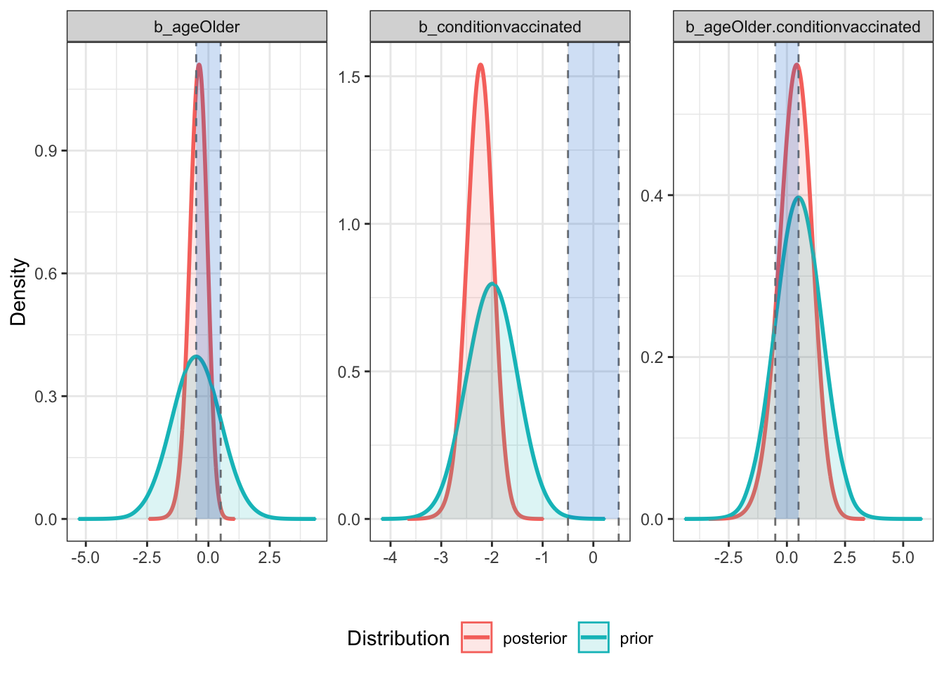
# bayestestR::sensitivity_to_prior(full_model, index = "Median", magnitude = 10)With “good” priors we can compare models
Now that we have convinced ourselves theoretically and by running the
full model that we have reasonable and informative priors we can
begin the process of comparing models. First step is to build
the other models by removing parameters and their associated
priors. Hopefully my naming scheme makes it clear what we’re
doing. The obvious and elegant thing to do would be to write
a simple purrr::map statement that would build a list of models
but for clarity I’ll simply repeat the same steps repeatedly (if
you want the purrr statement add a comment in disqus). I’ll
spare you printing all the various model summaries.
# no priors here
null_model <-
   brm(data = agg_moderna_data,
       family = binomial(link = logit),
       got_covid | trials(subjects) ~ 1,
       iter = 12500,
       warmup = 500,
       chains = 4,
       cores = 4,
       seed = 9,
       save_pars = save_pars(all = TRUE),
       file = "null_model")

# no prior for the interaction term
my_priors2 <- c(prior(normal(-0.5, 1), class = b, coef = ageOlder),
            prior(normal(-2.0, .5), class = b, coef = conditionvaccinated))

no_interaction <-
   brm(data = agg_moderna_data,
       family = binomial(link = logit),
       got_covid | trials(subjects) ~ age + condition,
       prior = my_priors2,
       iter = 12500,
       warmup = 500,
       chains = 4,
       cores = 4,
       seed = 9,
       save_pars = save_pars(all = TRUE),
       file = "no_interaction")
# summary(no_interaction)

# No prior for interaction or vaccine
my_priors3 <- c(prior(normal(-0.5, 1), class = b, coef = ageOlder))

no_vaccine <-
   brm(data = agg_moderna_data,
       family = binomial(link = logit),
       got_covid | trials(subjects) ~ age,
       prior = my_priors3,
       iter = 12500,
       warmup = 500,
       chains = 4,
       cores = 4,
       seed = 9,
       save_pars = save_pars(all = TRUE),
       file = "no_vaccine")
# summary(no_vaccine)

# no prior for interaction or for age
my_priors4 <- c(prior(normal(-2.0, .5), class = b, coef = conditionvaccinated))

no_age <-
   brm(data = agg_moderna_data,
       family = binomial(link = logit),
       got_covid | trials(subjects) ~ condition,
       prior = my_priors4,
       iter = 12500,
       warmup = 500,
       chains = 4,
       cores = 4,
       seed = 9,
       save_pars = save_pars(all = TRUE),
       file = "no_age")
# summary(no_age)
Okay, we now have models named full_model, no_interaction, no_age, no_vaccine, and
null_model. What we’d like to know is which is the “best” model, where best is
a balance between accuracy and parsimony. Highly predictive but doesn’t include
any unnecessary predictors. There are a number of ways to accomplish this including AIC and BIC
and even comparing R squared but we’re going to focus on
comparing Bayes Factors.
Using bayestestR::bayesfactor_models we’ll compare all our models to the null_model.
Then since as usual the null_model is a rather silly point of comparison we’ll
use update to change our comparison point to the model that does NOT include
the interaction term (a common question in research). That will help us understand
whether we need to worry about whether the vaccine is less effective in older subjects.
To make your workflow easier I actually recommend skipping this manual update process
and going straight to bayestestR::bayesfactor_inclusion(comparison, match_models = TRUE).
comparison <-
   bayestestR::bayesfactor_models(full_model, no_interaction, no_age, no_vaccine,
                                  denominator = null_model)
comparison
## # Bayes Factors for Model Comparison
##
## Model BF
## [1] age + condition + age:condition 7.352e+18
## [2] age + condition 9.708e+18
## [3] condition 1.991e+19
## [4] age 0.486
##
## * Against Denominator: [5] (Intercept only)
## * Bayes Factor Type: marginal likelihoods (bridgesampling)update(comparison, reference = 2)## # Bayes Factors for Model Comparison
##
## Model BF
## [1] age + condition + age:condition 0.757
## [3] condition 2.051
## [4] age 5.006e-20
## [5] (Intercept only) 1.030e-19
##
## * Against Denominator: [2] age + condition
## * Bayes Factor Type: marginal likelihoods (bridgesampling)bayestestR::bayesfactor_inclusion(comparison, match_models = TRUE)## # Inclusion Bayes Factors (Model Averaged)
##
## Pr(prior) Pr(posterior) Inclusion BF
## age 0.4 0.263 0.488
## condition 0.4 0.801 1.993e+19
## age:condition 0.2 0.199 0.757
##
## * Compared among: matched models only
## * Priors odds: uniform-equal### This is possible but NOT recommended
# bayestestR::bayesfactor_inclusion(comparison)There is very little evidence that we should include age or the
age:condition interaction terms in our model. If anything we have modest
evidence that we should exclude them! Weak evidence to be sure but evidence
nonetheless (remember bayesian inference allows for “supporting” the null,
not just rejecting it).
More elegant testing (order restriction)
Notice that our priors are unrestricted - that is, our \(\hat{b}_n\) parameters in the model have some non-zero credibility all the way out to infinity (no matter how small; this is true for both the prior and posterior distribution). Does it make sense to let our priors cover all of these possibilities? Our priors can be formulated as restricted priors (Morey, 2015; Morey & Rouder, 2011).
By testing these restrictions on prior and posterior samples, we can see how the probabilities of the restricted distributions change after observing the data. This can be achieved with bayesfactor_restricted(), that computes a Bayes factor for these restricted model vs the unrestricted model.
Think or it as more precise hypothesis testing. We need to specify these restrictions as logical conditions. An easy one is that I’m very confident that the vaccine is highly effective and \(\hat{b}_{conditionvaccinated}\) should be no where near 0. As a matter of research I want to know how the data support the notion that is less than -2 or a very large effect. How does that belief square with our data? More complex but testable, is that \(\hat{b}_{ageOlder.conditionvaccinated}\) (the interaction) if it is non zero is quite modest. The vaccine may work a little better or a little worse on older people but it is not a big difference.
chuck_hypotheses1 <-
   c("b_conditionvaccinated < -2")

bayestestR::bayesfactor_restricted(full_model, hypothesis = chuck_hypotheses1)
## # Bayes Factor (Order-Restriction)
##
## Hypothesis P(Prior) P(Posterior) BF
## b_conditionvaccinated < -2 0.497 0.822 1.654
##
## * Bayes factors for the restricted model vs. the un-restricted model.chuck_hypotheses2 <-
c("b_conditionvaccinated < -2",
"(b_ageOlder.conditionvaccinated > -0.5) & (b_ageOlder.conditionvaccinated < 0.5)"
)
bayestestR::bayesfactor_restricted(full_model, hypothesis = chuck_hypotheses2)## # Bayes Factor (Order-Restriction)
##
## Hypothesis
## b_conditionvaccinated < -2
## (b_ageOlder.conditionvaccinated > -0.5) & (b_ageOlder.conditionvaccinated < 0.5)
## P(Prior) P(Posterior) BF
## 0.499 0.822 1.648
## 0.340 0.444 1.305
##
## * Bayes factors for the restricted model vs. the un-restricted model.Although the support is limited (remember we had very few older subjects who got COVID-19) we at least have limited support and as our numbers continue to expand over the coming months we can continue to watch the support (hopefully grow).
Done
Hope you found this continuation of the series helpful. As always feel free to comment. Personally I find it helpful to work on real world problems and if you can follow these methods you’re in great shape in the next few months as more data becomes available to build even more complex models.
Keep counting the votes! Every last one of them!
Chuck

This work is licensed under a Creative Commons Attribution-ShareAlike 4.0 International License